Tag Archives: Excel

Create a Drop-Down List in Excel with Data Validation

Need to have consistency for a column of text that might be names, products, departments, countries, or some such? Your hunt is over…Create a drop-down list in Excel with Data Validation!

Columns of text for Data Validation

Control What Gets Typed in a Cell

You can end up with a mish-mash of abbreviations or spellings if you are typing them in on the fly or even worse, if others are filling in the data as their entries can further add to the problem.

Well, not to fret, Excel has you covered with a feature in Data Validation which allows you to create different types of lists. A simple drop-down list can be typed directly into the dialog box or if you already have it typed somewhere in your workbook, you can capture it and avoid retyping.

How to Create a Drop-Down List in Excel with Data Validation

Let’s cover some ways to create that list…

Important Prep: Select the column or range of cells where you want the drop-down list to display:

  1. On the Data tab, click Data Validation in the Data Tools group. The Data Validation dialog box will display:

    Data Validation Settings box

  2. On the Settings tab, select List from the Allow: drop-down box which will add the Source field.
  3. In the Source box, either:

    1. Type the names of the employees, departments or whatever your list is and separate each entry with a coma such as: Marketing, Human Resources, Administration OR
    2. If you have the list already typed somewhere in your workbook, click in the Source box and select the list. Example…if it is in Sheet 2 in A2:A6, click Sheet 2 and highlight that range and it will auto input as =Sheet2!$A$2:$A$6. The drop-down list of department names has now been created.*
    3. Click OK.


In your worksheet, click on any cell in the column (or range) with Data Validation and a drop-down arrow will display at the right of the cell. Users are forced to click the icon and choose from the list, and If anything is typed in the cell, an error message is displayed. You have the power!

Note: The two other tabs in Data Validation are important for different types of validation but not needed here as the drop-down list is self-explanatory. Because the default setting is Stop! in the Error Alert tab the user must select from the list.

*Named Ranges for Fast List Creation

An even faster method to create a list is to select the range with the names before opening Data Validation. Click in the Name box and type a name for the list, i.e., Dept and press ENTER. Open Data Validation and in the Source box, just type =Dept and click OK and  your drop-down list is created. This is called a Range Name (or Named Range).

Want to know more about how Named Ranges (Range Names) can be used in formulas and save time and effort? See my blog: https://gaylelarson.com/use-range-names-in-formulas/

Microsoft also has a detailed article and video tutorial for Data Validation lists at: https://support.office.com/en-us/article/Create-a-drop-down-list-7693307A-59EF-400A-B769-C5402DCE407B

Thanks for reading. Has Data Validation made your spreadsheets a lot cleaner and efficient to use? Let me know in the Comments!
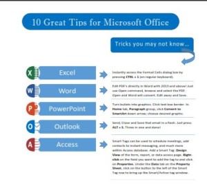
How to Find Cells that Contain Conditional Formatting

Applies to MS Excel 2007+

Find Cells that Contain Conditional Formatting

If you have applied Conditional Formatting in your workbooks, you may later want to know how to find cells that contain Conditional Formatting as it isn’t always obvious how the feature has been used or what the formatting represents. This is especially true if someone else created the file and now you need to work on it.

Colored numbered balls represent Conditional Formatting

Fortunately, it is relatively easy to find which cells have conditional formatting applied to them using the Go To feature of Excel.

Steps to find all conditional formatting:

1. Press F5 function key. Excel displays the Go To dialog box.

Excel Go To dialog box

2. Click Special… button to display the Go To Special dialog box.

Excel Go To Special... dialog box

3. Click on Conditional Formats 

4. Click OK

Excel now reveals all the cells in your worksheet that contain conditional formatting.

If that’s all you needed, you are free to go to lunch! If you want to see, edit or delete those formats, then read on…

How to See Existing Conditional Formatting Rules

Now that you know which cells contain conditional formatting, you might want to look at the definition of the different rules applied.

On the Home tab, Styles group, Conditional Formatting, Manage Rules:

Conditional Formatting Rules List

Select This Worksheet from drop down list to display all Conditional Formatting Rules for the worksheet:

Condiitonal Formatting Rules Manager dialog box

Click on Edit Rule… button to see details and what rule was applied or Delete Rule to remove it.

The Fast Way to Delete Existing Conditional Formatting Rules

You don’t have to be in the Rules Manager to delete any or all the conditional formatting applied, for instance…

If you want specific cells/ ranges cleared, select them first, then:

On the Home tab, Styles group, click Conditional Formatting, Clear
Rules > Clear Rules from Selected Cells

Conditional Formatting Clear Rules list options

To delete all the conditional formatting on the worksheet, you don’t need to have any particular cell selected, just choose > Clear Rules from Entire Sheet

Thanks for reading! Hope this has been valuable to you. For more helpful tips on Conditional Formatting and other neat Excel features, give a click and go to this blog: https://gaylelarson.com/conditional-formatting-clarity-visual-impact-excel/ 

Conditional formatting has six rules that can be applied to your data. For more information, visit this Microsoft site for additional options with this powerful tool:

Use Conditional Formatting to Highlight Text

Please leave a comment below and let me know how Conditional Formatting works for you in Excel…Happy Computing!

Analyze or Compare Workbook Versions with Spreadsheet Inquire

Analyze or Compare Workbook Versions with Spreadsheet Inquire is available with  Microsoft Office 365 or Office Professional Plus 2013 installed on your computer.

Note Spreadsheet Inquire was previously called Spreadsheet Compare.

What does Spreadsheet Inquire do?

You will want to analyze or compare workbook versions with Spreadsheet Inquire. You can also examine a workbook for problems or inconsistencies, or see links between workbooks or worksheets. Use the commands on the Inquire tab to do all these tasks, and more.

Where do I find the Spreadsheet Inquire feature?

The Inquire tab on the Excel ribbon has several groups and icons for the commands described below, and by default should display to the right of your last ribbon tab:

Spreadsheet Inquire on Excel ribbon

If you don’t see the Inquire tab in the Excel ribbon, it may not be activated…

How to turn on the Inquire add-in

If the Spreadsheet Inquire tab does not display in the ribbon, you may need to activate the add-in:

  1. Click File > Options > Add-Ins.
  2. Make sure COM Add-ins is selected in the Manage box and click the  Go… button.

  3. In the COM Add-Ins dialog box, make sure the box next to Inquire Add-in is selected.
  4. Click OK.

COM Add-in dialog box

After the add-in is turned on, the Inquire tab will appear in Excel.

Note    If you don’t see an entry for Inquire Add-in in the COM Add-Ins dialog box, it’s because either your version of Office or Excel doesn’t include it, or your organization’s system administrator has made it unavailable. Microsoft Office Professional Plus 2013 includes the Inquire add-in for Excel as does Office 365.

Compare two workbooks

Spreadsheet Inquire compares workbooks. The Compare Files command lets you see the differences, cell by cell, between two workbooks. You will need to have two workbooks open in Excel to run this command.

Results are color coded by the kind of content, such as entered values, formulas, named ranges, and formats. There’s even a window that can show VBA code changes line by line. Differences between cells are shown in an easy to read grid layout, like this:

Results of comparing two workbooks

The Compare Files command uses Microsoft Spreadsheet Compare to compare the two files (recent updates may say Spreadsheet Inquire):

  1. In Windows 8, you can start Spreadsheet Compare outside of Excel by clicking Spreadsheet Compare on the Apps screen.
  2. In Windows 7, click the Windows Start button and then > All Programs > Microsoft Office 2013 > Office 2013 Tools > Spreadsheet Compare 2013.

To learn more about Spreadsheet Compare and comparing files, read Compare two versions of a workbook.

Analyze a workbook

The Workbook Analysis command creates an interactive report showing detailed information about the workbook and its structure, formulas, cells, ranges, and warnings. The picture here shows a very simple workbook containing two formulas and data connections to an Access database and a text file.

Results of Workbook Analysis command

There are other features available in Spreadsheet Inquire. Be sure to look into them and let me know how you are using this useful add-in! More information at:   What you can do with Spreadsheet Inquire

Note
Many of  these screenshots are from the Microsoft website.

Want more ways to analyze or compare workbooks or worksheet data? Have a look at this post…

https://gaylelarson.com/5-amazing-must-have-excel-tips/ 

Let me know in the comments below if you have used some of the new Spreadsheet Inquire tools. Happy computing!

5 Steps for a Successful PivotTable

Trying to get more information out of that large spreadsheet? Functions such as VLOOKUP and SUBTOTAL are great summary tools but if your data changes frequently or you want to look at it in different ways, these 5 steps for a successful PivotTable will help you get great results.

PivotTable Numbers Picture

Why Use a PivotTable?

PivotTables allow you to look at your data in a variety of ways that aren’t possible in the regular grid format of a worksheet. Set up properly, you can also instantly access “underneath” details that automatically display on a separate worksheet.

Prepare Data for PivotTables

You only get out of PivotTables what you put into them, so there are some key points to follow before clicking that Insert button to get the best results and avoid errors.

5 Steps to a Successful PivotTable start with making sure all the data is in the rawest form:

  1. Remove any blank columns or rows.
  2. Need a header row with a name in each column in the first row of the data. (Each column name becomes a field in the PivotTable). Always a good idea to format the row bold or italic to distinguish it from the data.
  3. Don’t mix data types in a column. You want only dates in Dates column, numbers in Sales column, text with text, etc.
  4. Don’t use detail data for column headings in source data, use “Year”, not “2020”, use “Month”, not “January”, etc.
  5. Convert the data range into an Excel Table before creating the PivotTable (not necessary but has added benefits). When rows are added to expand the original worksheet table, the PivotTable will automatically update to include them when you click Refresh. If created from a regular worksheet range, only data edited within that range gets updated in the PivotTable.*

Here’s a worksheet I converted to a Table:

Excel Table Picture

Create the PivotTable

As a result, your worksheet is ready for primetime and creating the PivotTable:

  1. Click anywhere in the body of the data (if only using portion of worksheet, select that range first).
  2. Choose Insert tab and click the PivotTable icon in Tables group, to display a dialog box with your data range automatically selected. Placing it on a separate worksheet is also selected. (Can choose on same worksheet here if desired).
  3. Click OK and your new PivotTable Sheet is created.

Based on the above sample worksheet, this is the created PivotTable:

New PivotTable Picture

The PivotTable is now waiting for you to drag and drop the fields into the four area boxes at the bottom. Text columns would go in either Columns or Rows boxes and values such as sales or counts would go in the Values box.

Tweak the PivotTable

Here’s the PivotTable results after dragging Products into Columns, Salesperson into Rows and Sales into Values:

PivotTable Created from Fields Picture

So now, from here you can add filters, create subsets of data, such as dragging Year below Salesperson in Rows box would display sales by year underneath each Salesperson, and so much more!

The main thing here is to start right with clean format and data so your PivotTable behaves. Make a copy of a worksheet and play. You will be amazed!

You can also use a great feature available since Excel 2010 called Slicers which are visual filters. A blog on this feature and more PivotTable wonders coming soon!

*Click here for my blog on Excel Tables:    https://gaylelarson.com/magic-excel-tables/ 


Inspect and Remove Sensitive Document Properties with Document Inspector

It may come as a shock to some just how much information Microsoft collects in Document Properties during the creation of a file. This blog reveals how to inspect and remove sensitive document properties with Document Inspector. We have enough to handle just getting the document to be correct and look the way we want to present it without worrying about broadcasting sensitive data!

Office collects personal data

There are positive uses for this information and even for creating our own custom Document Properties, but we’ll cover that in a future blog as this is about protecting your information in Word, Excel and PowerPoint.

If the document is not leaving your computer or office, it may not be an issue to have unexpected details revealed about the creation path and timeframe for editing, how many revisions and more. On the other hand, if this is confidential or going to another department, or worse yet, to a client or outside organization, there could be a problem Houston!

NOTE: Document Inspector tends to be an all or nothing thing. Might want to create and save a copy of the document before you inspect, remove and send, because it may remove elements that you want to keep in your original.

What Data is Collected

As you work, here is what starts to accumulate about your document and you (or the user who is working on it).

Click File tab to display the Info screen (Backstage) with the Properties of the current document (left screenshot):

Word Document Properties

Much of the data is what you would expect to see if you were looking at the file in a directory, but note there are fields such as Total Editing Time, Author, Last Modified, Last Printed (and by whom).

If you click the link for Show All Properties at the bottom of the screen, you see more information is revealed such as Company and Manager (shown on the screenshot on the right). There are also several fields where you, the user, can enter details to identify the file for searching and clarity.

Let’s go one step further…At the top of the Properties column (in either screen), click the dropdown arrow and then click Advanced Properties button:

The Advanced Properties dialog box will display with five tabs that collect different data:

  1. The General tab contains the information you would see with the Details view in a directory.
  2. The Summary tab is where you can choose to add your own information to identify and describe the document.
  3. Statistics tab contains some file details but adds personal data about the construction of the file.
  4. The Contents tab pulls document properties from fields. For example, if you added a Title in the Title tab, it will appear here.
  5. The Custom tab is where you can add properties from the list such as Department or Editor or create your own.

As mentioned, you may want to utilize these properties for various reasons but, for now, we’ll just concentrate on what Word is collecting and tracking, and how to get rid of the information, if needed.

Note: Previously you could display the Document Panel from Advanced Properties directly at the top of your document and fill in the property tags there. It was removed from Office 2016.

Review with Document Inspector

Let’s look at all the document and personal information being collected:

  • Click the File tab and ensure Info is selected.

Inspect Document screen

  • Click Inspect Document under the Check for Issues dropdown arrow.
  • The Document Inspector displays where you can choose what content to check for.
  • Leave them all checked and click the Inspect button at the bottom of the dialog box.

Document Inspector dialog box pre-run

The same list displays again with the requested data flagged with a red exclamation mark and a list of the information found.

Document Inspector after running

Remove Hidden Data

If you want that data deleted, click the Remove All button. Click Reinspect to ensure it is gone or remove other information.

You can now send that file without fear that it is revealing your inner most document secrets, but you might want to take it one step further if the document has ever been shared, or you have cropped images! (See below).

Document Properties in Excel and PowerPoint

Both these programs use the same method for collecting data about your file but because of their diverse purposes, track some different information. You inspect and remove the same way with the Document Inspector.

Like Word, Excel and PowerPoint collect data on:
  • Comments, and Annotations
  • Document Properties and Personal Information.
  • Invisible Content
  • Custom XML Data
Excel adds:
  • Headers and Footers
  • Hidden Rows and Columns
  • Hidden Worksheets
PowerPoint adds:
  • Off-slide Content
  • Presentation Notes
 Word adds:
  • Revisions and Versions,
  • Metadata, Microsoft SharePoint properties, custom properties, and other content information.
  • Headers, Footers, and Watermarks
  • Hidden Text
  • Task Pane add-ins

How to Inspect and Remove

The same for all programs. Go to File | Info |Check for Issues | Inspect Document.  Note the list of things that will be inspected, leave them all selected and click the Inspect button.

Check Before Sending

There are some things not covered by the Document Inspector that could cause embarrassing or legal issues if the original information remained intact. Cropped images may display as you edited in the document, but the complete original image remains unless deleted. Same is true of Tracked Changes that have been edited if someone turns on All Marks.

Delete Cropped Areas of Images

  • Click on an image
  • In the Picture Tools | Format tab | Adjust group, click Compress Pictures

Compress pictures and delete cropped areas

  • Ensure there is NO checkmark in Apply only to this picture.
  • Ensure there IS a checkmark in Delete cropped areas of pictures.
  • Click OK.

Remove Tracked Changes

Accept or reject tracked changes to remove them from your document:

  • To look at each revision one at a time, on the Review tab, click Next in the Changes group, and then Accept or Reject.

Use Ribbon to remove tracked changes

Word keeps or removes the change and then moves to the next tracked change.

  • To accept all the changes at the same time, click the arrow below Accept, and then click Accept All Changes.
  • To reject all the changes at the same time, click the arrow below Reject, and then click Reject All Changes.

IMPORTANT:  Choosing the No Markup view helps you see what the final document will look like, but it only hides tracked changes temporarily. The changes are not deleted, and they’ll appear again the next time someone opens the document. To delete the tracked changes permanently, you’ll need to accept or reject them.

Whew! Now your clean and lean document can be sent without all that hidden data. If you want more information on security for your Office files, see the related blogs…

https://gaylelarson.com/word-document-protection/

https://gaylelarson.com/delete-personal-content-from-public-computers/

Have you had any surprise experiences with sharing sensitive information? Let me know in the Comments.


Use Excel Name Box for Navigation and Selection

In a previous post we covered navigating in Excel using the Name Box by typing a cell reference or a name for a cell or range of cells in the box or using the Go To dialog box (see link below).

compass for navigating your worksheet

When you name cells, they are called Range Names and become much more powerful, or at least more convenient, compared to using cell references.

Name Box for Navigation

The box reflects the current, active cell but does so much more. Although it looks separate, it is really part of the Formula Bar, so if you hide the Formula Bar, it disappears also.

The Excel Name Box

A quick recap on accessing the Name Box. There is no keyboard shortcut for landing there but you can press F5 function key to display the Go To… Dialog box and type in a cell reference in the Reference box; press ENTER or click OK, to go directly to that cell.

The Go To Dialog Box

Name Box for Selection of  Cell Ranges

Selecting huge ranges of data can be frustrating but if you know the cell references for the desired selection, the Name Box is the way to go. Just type in the range (or as close to it as you remember), i.e., a150:r8765, press ENTER, and that entire range is highlighted.

Tip: If you forgot column(s) or row(s) or included too many, just use SHFT and arrow keys to add or remove them. (Beats re-selecting two or three times).

Create Range Names in Name Box

The real power of the Name Box is to use it to create a name or ID for an often-used cell or range of cells, such as Commission or Regions, etc. You can create names that refer to cells, formulas, or a specific value.

The names can then be used for quick navigation or in a formula instead of cell references. You can create as many named ranges as desired and they are accessible from any worksheet in that workbook.

Steps to create range names:

  • Select the cell(s) that you want to name
  • Click in the Name box
  • Type a name for the cells (descriptive but short). There are some rules for range names:
    • Must start with a letter or an underscore
    • No spaces (can use an underscore to represent a space) *
    • Name may contain letters and numbers and periods but nothing that could be mistaken as a cell reference (examples: C, 2, R7C4)
    • Not case sensitive
    • Is ABSOLUTE cell referencing by default
    • Press ENTER after naming you range

 * Examples of naming a range could be: TotalSales or Total_Sales

Range Name example

Note: If there is a formula in that cell, it displays in the Formula Bar and the applied name in the Name Box.

I can now be anywhere in my workbook and return to that range with a click on the dropdown arrow in the Name box:

Name box with cell name

Now I don’t need to know the cell reference or even where it is located and can use that name in a formula, either for part of the formula or with other range names. For instance, if I had a commission rate in F8 and had named that cell, my formula would be: =TotalSales*Commission from any cell in my workbook. How sweet is that!

Name Box Limitations

There are several ways to create named ranges but the Name Box is the quickest. Be aware though that you can only create range names here, you cannot edit or delete them. That must be done from the Formulas tab on the Ribbon. You can also have Excel create range names for you using existing row and column labels to name them (covered later).

See original post for ways to navigate your worksheet:   https://gaylelarson.com/quick-navigation-excel-worksheet/

See the blog on Using Range Names in Formulas for more ways to use this great feature!  https://gaylelarson.com/use-range-names-in-formulas/

Are you liking this handy Name Box? Let me know in the Comments below!

Use Excel Sparklines Instead of Charts to Display Data Trends

What are Sparklines?

Sparklines were introduced in Microsoft Excel 2010 and add a quick way to display results without having to insert an entire chart object. A sparkline displays a visual representation of data as a tiny chart inside a single cell, and can be used to show trends in a series of values, such as sales for a company, products, sales representatives, time frames, economic cycles, or pretty much anything that has discernible increases or decreases.

Is a Sparkline a Chart Object?

The tiny sparkline chart actually resides in the background of a cell and displays a separate result in each cell for the range selected, unlike the chart object that displays all results in a single chart, such as a column, bar, pie, or a myriad of other chart types.

There are three different sparkline chart types, found on the Insert tab:

Sparklines Group

Create a Sparkline Chart

Because sparklines live in the background of a cell, you can insert them anywhere on your worksheet. However, people wouldn’t have a clue what they were supposed to represent as the Formula Bar is blank for any cell that contains a sparkline, unless you enter something else in the cell. Ergo…Best to put them next to your data.

Sparklines are automatically grouped by default but you can ungroup them to treat the cells separately. When you insert the chart, you can click in the first cell where you want the chart, and then select the rest of the range when inside the dialog box, or easier method, select the range first, and it will be auto displayed in the box:

Range to insert Sparklines

Click Insert tab to display the dialog box. If you have selected all the cell references for results, the Location Range is filled in and the Data Range: box is waiting for you to select the value cells:

Create Sparklines dialog bocx

Select the full range with the mouse of the values you are charting (in this case, B4:E8):

Data range for Sparklines

Click OK to insert the mini-charts.

Line Sparklines inserted next to data

Note: If you only selected the one cell, F4, when you inserted the sparkline, you can use the Fill Handle to populate the rest of desired cells. (You must drag the handle down though as the double click shortcut will not work here).

The Design Tab for Sparkline Tools

You don’t have all the fancy trappings of actual Excel chart objects but, hey, these are pretty spiffy and sometimes can even get the picture across in a clearer manner. The Sparkline Tools tab gets added to the end of the Ribbon and gives you many options for editing and formatting those little gems through the Design tab.

Sparklines Tools Design tab on Ribbon

You probably noticed that no markers displayed on the line charts but you can easily add them. (They are available only on this chart type). In the Show group, just click in the Markers box, and there you go – a marker for each change in value. Now you can use the Style group to choose a quick color change or individually change the Sparkline Color or Marker Color. (See below). Individual markers are also available for any chart type to represent High, Low, Negative, etc., in the Show group.

You can apply a color scheme to your sparklines by choosing a built-in format from the Style gallery or change your chart type from the Design tab (available when you select a cell that contains a sparkline). You can use the Sparkline Color or Marker Color commands to choose a color for the high, low, first, and last values (such as green for high, and orange for low).

Whatever selections you make are applied to all the sparkline cells as they are grouped by default. If you want to personalize a particular cell, or all cells individually, they can be ungrouped, and you can also type a comment directly in the cell without deleting the chart.

Ungroup Sparklines

Ungroup all the sparklines by selecting  that range, and choosing Ungroup from the Group group. (I’m not stuttering, honest)! If you just want to personalize one cell, select it, and choose Ungroup.

Sparkline cell with text entry

Using Sparklines for Stock Performance

This image shows a column sparkline in cell F2 and a line sparkline in F3. Both of these sparklines get their data from cells A2 through E2 and display a chart inside a cell that shows the performance of a stock. The charts show the values by quarter, highlight the high value (3/31) and the low value (12/31), show all the data points, and show the downward trend for the year. The high value marker is green, and the low value marker is orange. All other markers are shown in black.

Stock Performance Sparklines

Cell F6 shows the 5-year performance for the same stock, but displays a Win/Loss chart that shows only whether the year had a gain or a loss. This sparkline uses values from cells A6 through E6.

Sparkline Benefits

Sparklines can be inserted next to the data and take up such little space. They also easily point out a pattern. Any edits to your data automatically update the chart so the changes to trends are instantly represented. They can be inserted for rows or columns of data, and type changed with a mouse click.

*Stock Performance image from Microsoft

Find Sparklines fascinating? What would you use them for? Leave a comment below!

If you like different graphical ways of displaying your data, check out my blogs on using the Camera tool in Excel:

Part 1… https://gaylelarson.com/use-excel-camera-tool-combine-objects-several-workbooks/

Part 2…https://gaylelarson.com/excel-camera-tool-part-2/

Copy and Paste Filtered Subtotals or Visible Cells Only in Excel

Copy and Paste Visible Cells Only (filtered data)

You have used one of several methods to hide some rows for filtered data, or created a table which auto applies filter icons for each column. Now you want to copy and paste just the visible data but discovered to your horror when you pasted to another location, it included the hidden rows!

Excel, Paste only Filtered Data

By default, Excel copies hidden or filtered cells in addition to visible cells. If you want only visible rows, here’s the steps:

  • Select the cell range that you want to copy.
  • Click Home tab, Find & Select in the Editing group and choose Go To Special
  • Click Special… button in the dialog box.
  • Click Visible cells only radio button and click OK.

Excel, Copy and Paste Filtered Cells Only

  • Click Copy in Clipboard group on Home tab (or press CTRL+C).
  • Click the upper-left cell of the desired paste area and click Paste (or press CTRL+V).

You have now achieved Nirvana!

Tip: You can also use the F5 Function key at Step 2 to bring up the Go To… dialog box and click the Special… button to get the same results.

Add the Icon for Select Visible Cells to the Quick Access Toolbar

Make this great solution even easier and faster by utilizing the Quick Access Toolbar (QAT):

  • Right click anywhere in the Ribbon and choose Customize Quick Access Toolbar… OR click the QAT dropdown arrow, and choose More Commands
  • From the Choose Commands From dropdown, choose All Commands.
  • Scroll down and click Select Visible Cells.
  • Click Add and then click OK to add to end of the QAT.
  • If desired, use the arrow boxes to change the icon’s position on the toolbar.

Now all you do is select the range, click the Select Visible Cells icon on the QAT, Copy and Paste – One and done!

Copy and Paste Only Subtotaled Rows

You’ve used the SUBTOTAL function to sum only filtered data and now want to copy and paste to another location. You assume the paste will include the visible subtotaled rows only – Surprise – not! You still need to use the Go To dialog box to accomplish this but if this is something you do often, apply shortcuts:

  • Select the range you want to copy. (Excel is actually selecting the hidden rows as well but this will get taken care of in the next steps).
  • Press F5 function key to display Go To dialog box.

Excel, Copy and Paste only Subtotaled, filtered Rows with Special...

  • Click the Special… button at the bottom of the dialog box.
  • Click Visible Cells Only to select only the visible cells in the selected range.

  • Click OK (or just hit ENTER key as OK is already selected).
  • Press CTRL C to copy the selected visible cells to the Clipboard.
  • Select a destination cell (can be on the same sheet, a different sheet, or on a new workbook).
  • Paste the range by pressing CTRL V. Excel copies only the subtotaled rows.

Now you can copy and paste only those cells or ranges YOU want.

Hope these tips have removed a little head-scratching from one of those features that we want to use on a regular basis but doesn’t always behave the way we expect!

Display Results of Formula Inside Cell During Creation

Would you like to see the values displayed when you are entering a formula but a little fuzzy on how to make that happen?

Get clarity displaying formula values in cell

There are times when you may want to examine the results of a complicated formula from others or as you are creating one inside the cell. This can save time and frustration and avoid the dreaded error message after you hit ENTER or TAB.

If you want to look at the results of a particular part of a formula as you type, or after you or someone else has entered it, use a couple of function keys to complete the process.

Display Formula Values During Formula Creation

Here is a simple example of how handy this can be where we are adding sales of only two of the products, adding fees and dividing by cost, with the formula being entered in H9:

=(B9+E9)*G9/F9

Example displaying formula values in the cell

If I want to know the value of G9/F9 before completing the formula, I can do this directly in the cell.

  1. In the results cell (in this case, H9), type the formula.
  2. Select the part of the formula whose value you want to see. Here, it would be G9/F9.
  3. Press F9. Excel replaces that part of the formula with its result.

Selected portion of formula displays values

If this is the correct result, press ENTER or TAB, and Excel completes the formula and moves to requested cell. You could also press ESC to return to your formula and stay in the cell. Be careful here. If you are creating, not editing a previous entry, ESC will revert to whatever the cell contents were prior to your entry (such as a blank cell).

Display Formula Values Editing Existing Formula

If the formula already exists and you want to display the value, the steps are the same except you need to be in Edit mode in the cell:

  1. Click in the cell and press F2 to edit the formula in the cell. *
  2. Select the part of the formula whose value you want to see (G9/F9).
  3. Press F9. Excel replaces that part of the formula with its result.

*Note: Since the content already exists, you could also double click in the cell to edit. Only difference is that F2 places your insert marker at the end of the contents, and wherever you double click, the insert displays at that point.

Use the Ribbon to Evaluate Formula

There is another way to evaluate a formula by each cell reference – Select the Formulas tab, Formula Auditing group and click on Evaluate formula icon to bring up the Evaluate dialog box.

Example of Evaluate Formula dialog box

Click Evaluate button to see formula results as you move through each cell reference. This is a great way to walk through a formula you are not too familiar with and/or someone else created and has you scratching your head.

Now you can know what is going on in your worksheet before you press Print or Send!

Let me know if you have used these features or how they can help you in the future…

The Excel Camera Tool, Part 2

Create a Dashboard Using Camera Tool

We saw in Part 1 how to add the Camera tool to the Quick Access toolbar and how to use it for capturing linked pictures that automatically update when the source data is changed.

Another great use for the Camera tool is to create dashboards. The pasted objects can be sized proportionately and positioned anywhere on a worksheet. Here’s an example of sales figures and a chart:

Dashboard Example

This can contain as many objects as you choose. Note that the location of the original data is displayed in the Formula Bar.

Arranging as images on a worksheet in a dashboard-like mode is also a great fix for printing all your related information on one page. If you had selected all your original data separately, even from the same worksheet, the Add to Print command would have to be used which would automatically print each addition on a separate page. This way, you can add images, move, size and print at will.

The Camera tool captures everything as an image, including values, color formatting, shapes, even the gridlines. Because it is an image, the Picture Tools | Format tab is displayed on the ribbon so anything you can do to a picture, you can do here, including sizing and rotating. Use the right click menu to quickly perform commands such as Crop:

Moving Original Data

The Formula bar displays the path of the original data and the cell references are absolute by default. This is terrific because if the original data gets moved to another area, your pasted pictures reflect that, and continue to display any updates. Should be automatic but be sure that the workbook name (if different) and worksheet name display as well as cell references. If your workbook and worksheet are named, could look like this:

The Paste Special Option

The Paste Special Linked Picture option is available in Excel versions 2007 and above. If you prefer Paste Special, you can access it from the drop down arrow on the Paste icon in the Clipboard group or by right-clicking over desired destination cell and mousing over the Paste icons:

Paste Special Linked Picture

Tip: If you like keyboard shortcuts, press: ALT-H-V-I to paste a linked image.

Paste Special Linked Picture and Camera Tool Restrictions

Not too many downsides to using the Camera tool but here’s some cautions:

  • Some users say that it does not work with Tables; that the data must be converted to a range, but I have not experienced that with newer versions. The table copies, pastes and updates.
  • If using formulas such as IF function with Camera tool, you must use Named Ranges, rather than cell references to maintain the update connection.

Note: The Copy command in the Clipboard group on the Home tab, contains a Copy as Picture… option. This is handy but know that it pastes an image but not a link. Use when you just want a snapshot of your data.

Grab the post for Part 1 hereCamera Tool Part 1

See – don’t even have to be a photographer! Take some pictures and play with dashboards. What did you create?