Tag Archives: Excel

Use the Excel Camera Tool to Combine Objects from Several Workbooks

Uses for the Camera Tool

There is a little known spiffy tool that has been available for a long time in Excel which allows you to take screenshots of data from multiple worksheets or workbooks and paste them in a separate workbook as objects with links to their original locations. This can include ranges, tables or charts. Even better, if the original object updates, so does the linked object on your “collector” worksheet.

Here’s a short video to give you a quick overview of what the Excel Camera tool can do for capturing data and objects from different areas:

Collect desired data on one worksheet

For instance, you want to know the sales or prices from workbooks saved in different locations. You have figures for sales reps and a corresponding chart in Workbook A, and expenses that you want to track in Workbook B. Someone else may be updating the data but because anything you copy and paste with the Camera tool is pasted as a linked picture, any changes made to original data will auto update your screenshots.

Print collected objects on one page

This is also a great way to collect different areas of the same or separate worksheets or workbooks for printing a variety of data on one page as you can resize and move the different objects anywhere on the worksheet.

Add Camera Tool to Quick Access Toolbar (QAT)

First things first…The Camera is not available on the Ribbon by default so needs to be added to the QAT with the Customize Quick Access toolbar command:

  • Click the drop down arrow at end of Quick Access Toolbar. Choose More Commands… (or right click on the Ribbon)
  • Choose All Commands from drop down arrow next to Choose Commands from:
  • Scroll down the alphabetical list and click Camera.
  • Click Add button to add to Quick Access toolbar.
  • Click OK button at bottom of dialog box to place the Camera icon at the end of the QAT.

How to Capture a Screenshot

Select a range, table or chart to activate the Camera tool. Note, if selecting a chart, select the cell above the top, left border of the chart and draw around it. When you release the mouse, the “marching ants” will be around the object as if you had used the Copy command:

  • Go to your destination; usually in another worksheet or workbook.
  • Click in the desired cell location and the linked picture will auto insert.
  • Move and size the object(s) as desired.

Similar Feature with Paste Special Linked Picture

The newer versions of Excel (2007+) have another feature which behaves the same as the Camera tool – the Paste Special Linked Picture. I still prefer the Camera tool as just clicking on the desired destination cell pastes the linked image, all ready for sizing and relocating but both work.

The Camera tool can also be used to create Dashboards. We’ll cover that and some of the other options in an upcoming blog.

Take a picture and let me know what you think!

Want more ways to use the Camera? See Part 2: Camera Tool Part 2
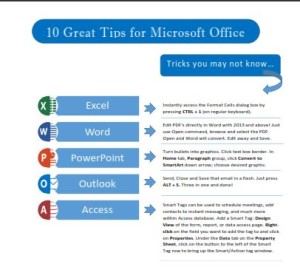
Conditional Formatting for Clarity and Visual Impact in Excel

Light Up the Cells with Conditional Formatting!

Conditional Formatting is a great tool for instant, visual results based on values, text or formulas in one or more cells. This is accomplished by creating rules for each desired result. It can be as simple as formatting all cells based on their values (the default), which could be applying a color in cell(s) that are above or below a certain value, contain specific text or fall within certain dates as well answer more complex questions.

Conditional Formatting is located on the Home tab | Styles group:

You can also choose to have the results displayed as Data Bars, Color Scales or Icon Sets (arrows or star ratings) instead of one solid color.

More than one condition can be applied to the same range of cells. This example below is returning two different results with two different cell colors based on two different questions (AND requires both conditions to be true but OR allows for either condition to be true to apply the rule).

The formulas in the last two columns have returned Yes or No based on True or False results. Range Names have been created from the header row text to make for easy identification of the cell references in the formulas. Then Conditional Formatting rules have been applied to designate the color(s) based on that answer.

=IF(AND(Years_Under_Contract<2,Number_of_Books_in_Print>4)=TRUE,”Yes”,”No”)

=IF(OR(Years_Under_Contract>5,Number_of_Books_in_Print>=10)=TRUE,”Yes”,”No”)

It is now very clear to see how many authors met none, one or both of the conditions.

Formatting Rules

There are four formatting rules applied here:

Rule Types

This is the Rule Type applied to the first rule for formatting only cells that contain “No” in the last two columns with Pink fill:


Each of the other three rules have their own Rule Description but all are based on Format only cells that contain (the second rule).

Note: You can include a formula directly in the condition by choosing the Rule Type: Use a formula to determine which cells to format and typing the formula in the Edit the Rule Description area.

Have you been using Conditional Formatting and, if so, which rule do you use the most? If not, I hope this post will encourage you to use this powerful feature. Thanks for reading!

Flash Fill in Excel 2013 and Above

Why You Need Flash Fill…

Flash Fill is a time-saving feature that reads patterns in adjacent columns and Lightening Flash
automatically fills the remaining cells in a column based on those patterns. It is useful when you need to join cells (Excel calls this Concatenate), or separate information in cells without wanting to write a cumbersome formula. You might already know the Text to Columns feature but this is faster and easier – Kind of like AutoFill on steroids!

Flash Fill should automatically be on by default but you can check here: File tab > Options> Advanced:


This amazing tool will make short work of many repetitive tasks, all without formulas (or the Text to Columns feature)! Just make sure you are working next to the column(s) you want to Flash Fill. Here’s just a few of the things it can do:

Splitting Input Data

You received a huge spreadsheet where someone has put first and last names in one column, and you need them separated for sorting and filtering. (This could be any data, i.e., department name and phone extension, or salesperson and monthly sales figure. Doesn’t matter as long as the data has a separator, such as a space). Flash Fill to the rescue…

Example: Full names are in Column A. Here’s the steps:

Insert:  two columns to right of Column A, and enter appropriate column header labels.

Type:  “Fred”, in appropriate cell ( B2 in example).

Press:  ENTER to go to cell below.

Type:  “Mary” (note that Excel has figured out what you are doing; displays the remainder of first names, and is awaiting your approval).

Press:  ENTER, and presto, all the rest of the first names are added!

Repeat the above steps in the cells for Last name (In example, C2)

List is now complete:

Just Want Last Names?

You can have flash fill complete only the last name, i.e., just insert one column, and instead of typing “Fred”, you would type “Frump”, ENTER, then “Lamb”, ENTER, and you would be done.

Combining Data

You can do the reverse of splitting data when you have or receive a workbook with data that is in two columns and you would like combined into one.

Example: Fred is in Column A and Frump in Column B:

  1. Insert a blank column to right of Column B.
  2. Type the first instance the way you would like it displayed, i.e., Fred Frump or Frump, Fred.
  3. Press ENTER and start to type the second example. Excel should display the preview for the balance of the column. Just press ENTER to complete.

You Mean Flash Fill Does More?

Give Excel one or two examples of what you are trying to accomplish so Flash Fill can see a pattern. It will work with text, email addresses, dates, numbers and time:

If Flash Fill does not appear to work when entering the second example, you can activate it from the Ribbon: Data  tab > Flash Fill or keyboard with CTRL E. Just click in the second cell (ensure blank) and use the Ribbon command to fill down the column.

ALERT: Be aware that if you change source data, cells containing flash fill data will not update as there are no formulas involved.

There are many other ways to use Flash Fill. Now that you can save all that time entering data, what ways will you use it?

Reasons to Format Excel Spreadsheets with Cell Styles

Use Cell Styles to Format in Excel to save time and frustration and look smart doing it!

Here’s why you want to use Cell Styles to format Excel data:

  • Apply professional formatting to a worksheet in a flash.
  • Consistency across worksheets.
  • Built-in styles are labelled according to purpose for easy use.
  • Styles are customizable so you can edit existing styles or create your own to match your needs.
  • One click formatting.

Have you ever wondered how to format a spreadsheet in a hurry? Here’s a simple example of a worksheet with boring, unformatted data:

Name Region Q1 Q2 Q3 Q4 Total
Smith South 21223 17855 24855 21377 85310
Jones Southwest 23456 29550 24294 25335 102635
Wing North 19954 22600 19448 26450 88452
Baker South 17564 25439 32944 24000 99947
Folsom North 28543 28540 24400 28550 110033
Range Northwest 19534 30558 21844 19605 91541
McKnight West 20585 29667 27595 13605 91452
Crump South 24957 31322 15330 27550 99159
Rogers North 30332 27407 26440 24007 108186
Morris East 25395 27700 16500 27500 97095
Rollins South 35822 31854 24384 31005 123065
Jefferson Southwest 20949 23100 21774 27550 93373

But now you get a call to send it to a co-worker or the boss or it has to be ready for a presentation. Using individual formatting tools, it can take longer to format than it took to create it!

Format the Column headers and Data Content

Want to look smart really fast? Here’s the fix…First, I want to format the header row:

Select the header row in the worksheet

On the Home tab, in the Styles group, click Cell Styles icon:

If you have a larger screen and/or higher resolution, you may see several cell styles already displayed. See all styles by clicking the More arrow button at the bottom of the scroll bar for the group.

This box below will display with lots of options that are labelled for specific uses but you can use them for any purpose you choose. Roll your mouse over the sections and because they are live preview, you can see the results before you actually choose the option. I want Heading 1 for my header row, so I point and click to apply it.

I’ve selected Heading 1 under the Titles and Headings section:

Next select the body of the spreadsheet:

Click Cell Styles again, and choose whatever style you think would look best for your data. (If you are using Input Style, don’t include the Total column as you’ll probably want to use the Calculate Style for that to indicate formulas).

Total Row Style

If you have a total row, quickly make your totals stand out with the Total Style:

Data and Model Section

A way to alert users about which data they can edit is to use the Input and Calculation styles under the Data and Model section. It can’t stop them from overwriting formulas, etc., but it does signify the ranges that they should not edit. If you don’t like the default colors, you can change them. (See below)

Remove Styles

So, you’ve been playing and got carried away and now your data looks like a kindergarten project! Don’t worry if you goof and want to remove a style. Just select that range of cells; go back to the Cell Styles icon to the Style group and click on Normal to reset the cells to your default font style and size. (Located in the upper left of the first section, Good, Bad
and
Neutral).

Customize/Create Styles for Text

You can modify any style or leave the original styles and create a duplicate for your new style. I would recommend the latter. Here’s how to make changes in font, color, etc. for any style:

Example here is for Heading 1:

  • Click the Cell Styles icon (Home tab, Styles group).
  • Right click over the style you want to change.
  • Choose Duplicate (or Modify if you want to edit the original style) to display the Style box:

  • Change the name.
  • Click the Format… button and make desired changes. (Ensure Font tab is selected).
  • Click OK, OK.

Changes to Numerical Data Styles

If you want to change the Input or Calculation or any other numerical styles to add number formatting as well, the process is the same except you:

  • Right click over the style name.
  • Choose Duplicate.
  • Type in a new style name.
  • Click on the Number tab in the Format Cells dialog box.
  • Click on Currency in the Category pane.
  • Choose if you want the style to always display 2 decimal places or change to 0 if you want that for the style.
  • Make any other desired changes to Font, Alignment, etc., using the tabs at top.
  • Click OK, OK.

Apply Customized Styles

This can be a little confusing after modifying a style as it looks like nothing happened. The new style is not applied to your selected data. because you have created the style but not yet applied it.

When you customize or create new styles, Excel adds a Custom section to the top of the Cell Styles list. Just select desired data, click Cell Styles and click on your customized style. I added Currency formatting to the Input Style but left the background cell color; applied Currency formatting for the Calculate Style but changed to red color so it would be obvious not to enter data in those cells:

I selected the quarterly data to apply my customized Input Style, and then selected the Total column to apply my new Calculation Style. If there is also a Totals row, I would select them both first, and then go to Cell Styles and click my customized style:

Create your own styles and save a bundle of time while looking darn professional as well!

Let me know how it works for you…

Quick Navigation in Excel Worksheets

Go There in a Flash in Excel

You inherited the biggest spreadsheet on the planet and have to scroll and troll to ranges miles away from your current screen! Don’t despair, Excel has several tools to get you there quickly…

The Go To Dialog Box

You can jump to any area of your worksheet with this handy command. Using the Ribbon, Home tab, Editing group, Find & Select drop down arrow, and select Go To… Just type in a cell reference, click OK or press ENTER, and you are there!

OK, that might beat scrolling but not by much, so here’s the corresponding shortcut:

Press CTRL G or F5 function key to auto display the Go To Dialog Box and it is ready for your entry. It also remembers your previous cell location(s).

The Name Box

Want the quick mouse navigation trick? The Name Box is your ticket! Just click in the box and type the cell reference (such as T44456); press ENTER and you are there. (Unfortunately, there is no keyboard shortcut for the actual Name Box but you could use F5 to display the Go To box, type the cell reference and press ENTER).

keyboard angled 2 x 3
Where did I put that?

Range Names

The amazing Name Box is multi-talented. We saw we can highlight large ranges of cells and also jump to a faraway cell location just by typing the cell reference(s) in the Name Box. But what if you are short on sleep and can’t remember the cell reference(s)? No problem. There is a reason it is called the “Name Box”. All you have to do is find that cell once, select it and give it a name that makes sense to you, like Sales or Profit, etc.

Steps:

  • Navigate to desired location
  • Click on desired cell (or range of cells)
  • Click in the Name Box and type a name, i.e., Sales
  • Press ENTER

To return to that location any time, just click the drop-down arrow on the Name Box and select the name you gave it, and you are magically transported there!

Important things to know when naming a cell:

  • Range Names must start with a letter but can contain numbers.
  • You can use more than one word to name a range but it cannot contain spaces.
  • Capitalize the separate words, like TotalSales, or the underscore can be used to represent the space, i.e., Total_Sales.

Range Names are ABSOLUTE by default, meaning the name will always refer to the cell even if the content is moved. And, even more impressive, Range Names can also be used in formulas instead of cell references. That Excel is one smart cookie!