Use Cell Styles to Format in Excel to save time and frustration and look smart doing it!
Here’s why you want to use Cell Styles to format Excel data:
- Apply professional formatting to a worksheet in a flash.
- Consistency across worksheets.
- Built-in styles are labelled according to purpose for easy use.
- Styles are customizable so you can edit existing styles or create your own to match your needs.
- One click formatting.
Have you ever wondered how to format a spreadsheet in a hurry? Here’s a simple example of a worksheet with boring, unformatted data:
But now you get a call to send it to a co-worker or the boss or it has to be ready for a presentation. Using individual formatting tools, it can take longer to format than it took to create it!
Format the Column headers and Data Content
Want to look smart really fast? Here’s the fix…First, I want to format the header row:
Select the header row in the worksheet

On the Home tab, in the Styles group, click Cell Styles icon:

If you have a larger screen and/or higher resolution, you may see several cell styles already displayed. See all styles by clicking the More arrow button at the bottom of the scroll bar for the group.

This box below will display with lots of options that are labelled for specific uses but you can use them for any purpose you choose. Roll your mouse over the sections and because they are live preview, you can see the results before you actually choose the option. I want Heading 1 for my header row, so I point and click to apply it.
I’ve selected Heading 1 under the Titles and Headings section:

Next select the body of the spreadsheet:

Click Cell Styles again, and choose whatever style you think would look best for your data. (If you are using Input Style, don’t include the Total column as you’ll probably want to use the Calculate Style for that to indicate formulas).
Total Row Style
If you have a total row, quickly make your totals stand out with the Total Style:

Data and Model Section
A way to alert users about which data they can edit is to use the Input and Calculation styles under the Data and Model section. It can’t stop them from overwriting formulas, etc., but it does signify the ranges that they should not edit. If you don’t like the default colors, you can change them. (See below)
Remove Styles
So, you’ve been playing and got carried away and now your data looks like a kindergarten project! Don’t worry if you goof and want to remove a style. Just select that range of cells; go back to the Cell Styles icon to the Style group and click on Normal to reset the cells to your default font style and size. (Located in the upper left of the first section, Good, Bad
and
Neutral).
Customize/Create Styles for Text
You can modify any style or leave the original styles and create a duplicate for your new style. I would recommend the latter. Here’s how to make changes in font, color, etc. for any style:
Example here is for Heading 1:
- Click the Cell Styles icon (Home tab, Styles group).
- Right click over the style you want to change.
-
Choose Duplicate (or Modify if you want to edit the original style) to display the Style box:

- Change the name.
- Click the Format… button and make desired changes. (Ensure Font tab is selected).
-
Click OK, OK.

Changes to Numerical Data Styles
If you want to change the Input or Calculation or any other numerical styles to add number formatting as well, the process is the same except you:
- Right click over the style name.
- Choose Duplicate.
- Type in a new style name.
- Click on the Number tab in the Format Cells dialog box.
- Click on Currency in the Category pane.
- Choose if you want the style to always display 2 decimal places or change to 0 if you want that for the style.
- Make any other desired changes to Font, Alignment, etc., using the tabs at top.
- Click OK, OK.

Apply Customized Styles
This can be a little confusing after modifying a style as it looks like nothing happened. The new style is not applied to your selected data. because you have created the style but not yet applied it.
When you customize or create new styles, Excel adds a Custom section to the top of the Cell Styles list. Just select desired data, click Cell Styles and click on your customized style. I added Currency formatting to the Input Style but left the background cell color; applied Currency formatting for the Calculate Style but changed to red color so it would be obvious not to enter data in those cells:
I selected the quarterly data to apply my customized Input Style, and then selected the Total column to apply my new Calculation Style. If there is also a Totals row, I would select them both first, and then go to Cell Styles and click my customized style:


Create your own styles and save a bundle of time while looking darn professional as well!
Let me know how it works for you…
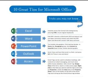 Click to download great tips to speed up your Office projects.