Microsoft announced it will retire Office Mix on May 1, 2018, but the best features of Office Mix will be integrated into PowerPoint 365 so it will no longer be an add-in download. This will also include Microsoft Stream and Forms for easier creation and sharing of interactive online videos for Office 365 users. It has something for everyone who wants tools for creating slick media from PowerPoint.

What is Office Mix and Should I Care?
Mix is a PowerPoint add-in that Microsoft introduced about three years ago and is/was available for Office 2013 and above. It is pretty amazing and looks to be even more so as a feature baked directly into PowerPoint. You can create presentations videos, screen recordings, narrations, ink and audio, to name a few features, and upload to the cloud for storing and/or sharing. You can also download the converted video to your hard drive or wherever if you choose. It is directed toward educators but available for anyone with a 365 account. It even includes interactive quizzes and simulations.
Note: See the link below to my earlier blog with an overview of Office Mix.
Most of the information below is from Microsoft and includes links to relevant pages and support a for transitioning from Mix to Stream if you are a current user, and how to access these great interactive tools if you want to start.
What do you need to do to prepare for this change?
If you have a qualifying account* and would like us to migrate your existing mixes to Microsoft Stream, please click here to visit the Office Mix migration page, sign in, and follow the prompts to automatically migrate your data. When the process completes, your mixes will be stored on Microsoft Stream as videos. You can continue to access Office Mix until May 1, 2018.
Mixes migrated to Stream will not include analytics data, quizzes or apps. However, over time these mixes will become interactive again. If you would like to save this content, you can download your mixes as PowerPoint files (.pptx), and your analytics data as Excel files (.xlsx) to save to your storage location of choice at any time before May 1, 2018. Please visit our help article for more details.
If you’re an Office Mix user, you can find full details on how to migrate your mixes ahead of the shutdown at Microsoft’s support page.
Migrate your content from Office Mix
Applies To: PowerPoint 2016
Just over three years ago we launched the Office Mix Preview to help everyone from educators to business create and share interactive online recordings of their presentations. Thanks to the positive feedback from our users during the Preview, we are excited to share that we are bringing the best of Office Mix directly into PowerPoint, Microsoft Stream, and Microsoft Forms for Office 365 subscribers on Windows PCs.
This new integrated experience in PowerPoint will remove the need for downloading an add-in. You’ll be able to easily access the feature via the Recording tab in PowerPoint after you turn on the feature by customizing your PowerPoint toolbar ribbon.
In the coming months, you’ll also be able to publish these recordings to Microsoft Stream, which offers a simple way to upload and share videos securely across your organization to improve communication, participation, and learning.
If you’d like us to migrate your existing mixes to Microsoft Stream, please click here to visit the Office Mix migration page, sign in, and follow the prompts to automatically migrate your data. When the process finishes, your mixes will be stored on Microsoft Stream as videos. You can continue to access Office Mix until May 1, 2018.
This article contains details on how to back up content you currently have on mix.office.com. Please note that all content must be moved off Mix by May 1, 2018, to avoid losing it. If you take no action by that date, your files will no longer be accessible. We will continually update this article as more information becomes available.
I’m a current Office Mix user—What does this change mean for me?
The Office Mix site and existing content stored on its servers will be retired according to the following schedule:
- October 20, 2017: If you have an existing Office Mix account, you’ll still be able to view, edit, publish, download, and delete your existing content. If you have a qualifying* Office 365 work or school account, you can sign in to migrate your mixes as videos to Microsoft Stream. If you don’t have access to an Office 365 work or school account, you can download your Mixes as PowerPoint files (.pptx), and your analytics data as Excel files (.xlsx) to save to a storage location of your choosing.
*Office 365 plan features vary by license. See licensing details to learn if you already have access to Microsoft Stream and what features you can use, or to upgrade your plan.
- January 1, 2018: You’ll no longer be able to sign up as a new user or download the Office Mix add-in from the website. Existing users who already have the Mix add-in installed will still be able to use it to upload, edit, view, and download their existing content.
- May 1, 2018: The Office Mix site and all its content will be officially discontinued. The site will no longer be accessible after that date. Any links to your Office Mix content that you previously shared with others will stop working after this date.
How do I move my files and content from Office Mix?
For Office 365 work or school accounts
Do the following:
- Please visit https://mix.office.com and sign in with your Office 365 work or school account that you were using for Office Mix.

- Click the Migrate button.
- On the confirmation page, click Migrate Now.

-
Once you click
Migrate Now, you’ll be asked to sign in by using your Office 365 account; after sign-in is successful, the migration will start for all Mixes in the “Ready for Migration” state. Migration may take some time to complete, and during migration you’ll be able to get status on the migration on the website. Please visit
https://mix.office.com again to confirm the results.

For Microsoft accounts (Outlook.com, Hotmail.com, Live.com, etc.) and Google and Facebook accounts
Do the following:
- Please visit https://mix.office.com and sign in with the account that you were using for Office Mix.
- Click My Mixes.
- Under the uploaded mixes page, click Presentation to download your mix as a PowerPoint file (.pptx). If you enabled mobile playback during upload, you may see a Video button that you can use to download a video (.mp4) of your Mix as well.
- To download your quiz results and analytics data, click Analytics and then click the Excel icon to download an Excel file (.xlsx). For more detailed instructions, see Export your analytics to Excel.
For Microsoft, Google, and Facebook accounts with access to a valid school email address
We can back up your mixes as videos to your Microsoft Stream account. All you need to get started is to enter a valid school email address. Please see Get Office 365 for Education for free. Students and teachers are eligible for Office 365 for Education, which includes Word, Excel, PowerPoint, OneNote, and now Microsoft Teams, plus additional classroom tools.
You can also choose to sign in to Office Mix and follow the auto-migration prompts yourself. When the process is complete, you will find all compatible content you had previously published to Office Mix backed up to your Microsoft Stream account. The original content on Office Mix will thereafter only be available to view, download, and delete.
Which Office 365 plans will include Microsoft Stream?
Stream is available currently to all the same plans that Office 365 Video was available in except (Government Community Cloud, Germany, and China).
These are the plans that include Stream:
- Office 365 Education
- Office 365 Education Plus
- Office 365 Enterprise K1
- Office 365 Enterprise K2
- Office 365 Enterprise E1
- Office 365 Enterprise E3
- Office 365 Enterprise E5
Over the course of time we will be adding Stream instances and licensing to match the existing set of regions and plans supported today by Office 365 Video.
For Office 365 Accounts without Microsoft Stream
Sign in to your Office Mix profile where you can download and save your content to your device or your preferred storage and sharing platforms. You can also delete your Office Mix account and content.
What about content that I have already linked from Office Mix to other Web sites?
For users who have embedded or shared content in a Learning Management System using the Office Mix LTI tool, you can embed content using Microsoft Stream. If you want to remove linked content, simply delete the files from your My Mixes page. On May 1, 2018, all Office Mix content and links will stop working, so please make sure to manually update any embedded Mixes on your other Web sites before this date.
What if my Office Mix content exceeds my Microsoft Stream upload storage limit?
If you exceed your available storage limit on Microsoft Stream, the migration of your Office Mix content will be interrupted. Any files that were successfully transferred will remain on your Microsoft Stream account, but any files that couldn’t be included won’t be backed up and the migration process will stop.
Content migration can be resumed after you have freed up or purchased additional storage space on your Microsoft Stream account. To resume an interrupted migration, sign back in to Office Mix and then start migration again. To learn more about the quotations and limitations for Microsoft Stream, click here.
I am an Office 365 Administrator. What do I need to know?
If you are an Office 365 administrator, you can share this article with your organization. Currently, we do not support migrating content from a tenant level, so each Office Mix account holder needs to sign in and migrate his or her own mixes.
When will the Recording tab come to PowerPoint for Mac?
Currently, the Recording tab is only available to Office 365 subscribers on Windows PCs. In the future we may consider rolling out these features to other platforms over time.
When will Microsoft Stream support interactive quizzes and analytics?
We are working to bring interactivity to the Microsoft Stream video player so you can build, upload, play back, and share more Mix-like content on Microsoft Stream (that includes quizzes, ability to jump to different parts of the presentation, and more). Over time, we’ll enhance the analytics capabilities for videos on Microsoft Stream. For more information about the current capabilities of Microsoft Stream, please click here.
How do I turn on the Recording tab in PowerPoint?
My Note: I have Office 365 (Educator edition), and the Recording tab automatically appeared on the Ribbon, with this notation:

If you have Office 365 and The Recording tab is not automatically on the Ribbon, follow these Microsoft instructions:
Turn on the Recording tab of the ribbon:
On the File tab of the ribbon, click Options. In the Options dialog box, click the Customize Ribbon tab on the left. Then, in the right-hand box that lists the available ribbon tabs, select the Recording check box. Click OK. For more information about the PowerPoint Recording tab, see Record a slide show with narration and slide timings.

How do I upload a video to Microsoft Stream?
You can find the upload button at the top of any page or just drag new videos to one of your groups or channels. You can upload multiple videos at the same time and even browse Microsoft Stream while your videos are uploading in the background. In the Microsoft Stream portal, select Create > Upload a video or the “upload” icon from the top navigation bar. Drag and drop or select files from your computer or device. For more information, see Upload a video.

I need more help!
If you’re unsure of what steps to take before the Office Mix service is retired, or you are encountering any issues during your content migration, please contact support at https://officemix.uservoice.com.
We sincerely appreciate your feedback and we’ll be happy to provide further assistance with this transition.
* Office 365 plan features vary by license. See licensing details to learn if you already have access to Microsoft Stream and what features you can use, or to upgrade your plan.
Thank you for using Office Mix and being on the journey with us. If you’re unsure of what steps to take before Office Mix is retired, or you are encountering any issues during your content migration, please visit our help article.
My Note: Here is the link to my previous post on Office Mix:
https://gaylelarson.com/share-powerpoints-office-mix/
Have you been using Office Mix? Tell me about your experiences and if you are going to take advantage of the new features!


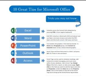 Click to download great tips to speed up your Office projects.